|
網路結構
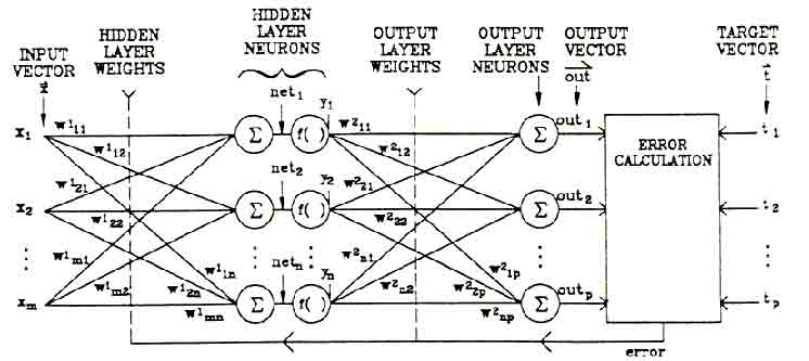
多層前饋式神經網路是一個層狀的前饋結構,分為輸入層(input
layer),隱藏層(hidden
layer),與輸出層(output
layer),每一層都包含許多處理單元。網路系統中的每個處理單元都和其下一層的所有處理單元連接,但是同一層內的處理單元都不互相連接。

使用Delta
Rule學習 神經網路輸出的誤差函數(Error
Function)定義為:

tj為網路所期待的輸出值;oj為網路的實際輸出值。倒傳遞學習的目標即在於使此誤差值(或稱為能量函數,E
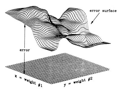
)達到最小。 如果只考慮神經網路的兩個鏈結權值:weight
#1和weight
#2,它們的值域分別定義在一個x-y平面上的x軸和y軸上,則我們可以表示誤差值為一個x、y變數的函式,如圖
 倒傳遞學習主要目的在於使輸出層之預測值與實際值的均方差最小化,而整個網路之加權值即依此目標作調整。 計算梯度(gradient) In order to train neural networks such as the ones shown above by gradient
descent, we need to be able to compute the gradient G of the loss
function with respect to each weight wij of the network. It
tells us how a small change in that weight will affect the overall error
E. We begin by splitting the loss function into separate terms for each
point p in the training data:
  |
(1) | where o ranges over the output
units of the network. (Note that we use the superscript p to denote the
training point - this is not an exponentiation!) Since differentiation and
summation are interchangeable, we can likewise split the gradient into separate
components for each training point:
  |
(2) | In what follows, we describe the
computation of the gradient for a single data point, omitting the superscript
p in order to make the notation easier to follow.
First use the chain rule to decompose the gradient into two
factors:
 |
(3) | The first factor can be obtained by
differentiating Eqn. 1 above:
 |
(4) | Using  , the second factor becomes , the second factor becomes
 |
(5) | Putting the pieces (equations 3-5)
back together, we obtain
 |
(6) | To find the gradient G for the
entire data set, we sum at each weight the contribution given by equation 6 over
all the data points. We can then subtract a small proportion µ (called
the learning rate) of G from the weights to perform gradient
descent.
(error-backpropagation詳細推導)
誤差倒傳遞學習演算法
We want to train a multi-layer feedforward network by gradient descent to
approximate an unknown function, based on some training data consisting of pairs
(x,t). The vector x represents a pattern of input to the network,
and the vector t the corresponding target (desired output). As we
have seen before, the overall gradient with respect to the entire training set
is just the sum of the gradients for each pattern; in what follows we will
therefore describe how to compute the gradient for just a single training
pattern. As before, we will number the units, and denote the weight from unit j
to unit i by wij.
- Definitions:
- the error signal for unit j:
|
|  |
- the (negative) gradient for weight wij:
|
|  |
- the set of nodes anterior to unit i:
|
|  |
- the set of nodes posterior to unit j:
|
|  |
- The gradient. We expand the gradient into two factors by use of the chain
rule:
The first factor is the
error of unit i. The second is
Putting the two together,
we get
 . To compute this gradient, we thus need to know the activity and the error for
all relevant nodes in the network.
- Forward activaction. The activity of the input units is determined by
the network's external input x. For all other units, the activity is
propagated forward:
Note that before the activity of unit i can be calculated, the activity of
all its anterior nodes (forming the set Ai) must be known. Since
feedforward networks do not contain cycles, there is an ordering of nodes from
input to output that respects this condition.
- Calculating output error. Assuming that we are using the sum-squared
loss
the error for output unit o is
simply
- Error backpropagation. For hidden units, we must propagate the error
back from the output nodes (hence the name of the algorithm). Again using the
chain rule, we can expand the error of a hidden unit in terms of its posterior
nodes:
Of the three factors inside the sum, the first is just the error of node i.
The second is
while the third is the derivative of node j's activation function:
For hidden units h that use the tanh activation function, we can make use of
the special identity
tanh(u)' = 1 - tanh(u)2, giving us
Putting all the pieces together we get
Note that in order to calculate the error for unit j, we must first know the
error of all its posterior nodes (forming the set Pj). Again, as long
as there are no cycles in the network, there is an ordering of nodes from the
output back to the input that respects this condition. For example, we can
simply use the reverse of the order in which activity was propagated forward.
學習速率的影響
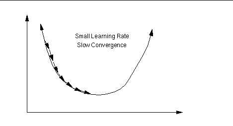
An important consideration is the learning rate µ, which determines by
how much we change the weights w at each step. If µ is too small,
the algorithm will take a long time to converge .
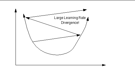
 Conversely, if
µ is too large, we may end up bouncing around the error surface out of
control - the algorithm diverges. This usually ends with an
overflow error in the computer's floating-point arithmetic. Conversely, if
µ is too large, we may end up bouncing around the error surface out of
control - the algorithm diverges. This usually ends with an
overflow error in the computer's floating-point arithmetic.

延伸閱讀
Improving the Backpropagation Algorithm(IEEE Trans. Neural Networks 8(3): 799-803. )
|
|
